satellite | Ocean Bytes Blog

Tag: satellite

Utilizing New Tagging Technology to Characterize Sand Tiger Shark Habitat

April 16, 2012 / Danielle / Comments Off

Sand tiger sharks are large bottom dwelling sharks found in the coastal waters of the Eastern North Atlantic, and are known to frequent the Delaware Bay in the summer months. Sand tiger shark populations are currently in danger of over exploitation because they are slow growing and have extremely low birth rates. While we know that the sharks are found within the Delaware Bay during summer months, little is known about their movements during the rest of the year, or what oceanographic conditions limit their spatial extent. There is evidence that these sharks make large coastal migratory movements along the Eastern Seaboard. This makes habitat characterization difficult because the sharks travel throughout such a large area. It is important for managers to know the areas of intensive use by the sharks, and the species assemblages within those areas, in order to protect these apex predators.

Dr. Matthew Oliver and Danielle Haulsee with a sand tiger shark caught in the Delaware Bay.

Our project, a collaboration among Delaware State University’s Dewayne Fox and the University of Delaware’s Matthew Oliver and Danielle Haulsee, will document and characterize the movements of sand tiger sharks, their habitat preferences, and the community assemblages they encounter using new and innovative electronic tagging technology. Sand tiger shark movements will be recorded using passive telemetry in addition to pop-off satellite archival tags. We will also deploy a new type of tagging technology, which acts as a mobile receiver, and will record any encounters with other sharks, fish or other marine animals that have been tagged with acoustic tags. We will then use satellite and remotely sensed data resources from the Mid-Atlantic Regional Association for Coastal Ocean Observing Systems (MARACOOS) to characterize and model the habitats and oceanographic conditions used by sand tiger sharks. This study will give managers a better understanding of the spatiotemporal patterns in sand tiger shark movements along the East Coast, as well as inform management decisions regarding sand tiger shark habitat utilization.

Predicting Sea Surface Salinity from Space

November 21, 2011 / dw / Comments Off

The simplest definition of salinity is how salty the ocean is. Easy enough, right? Why is this basic property of the ocean so important to oceanographers? Well, along with the temperature of the water, the salinity determines how dense it is. The density of the water factors into how it circulates and mixes…or doesn’t mix. Mixing distributes nutrients allowing phytoplankton (and the rest of the food web) to thrive. Globally, salinity affects ocean circulation and can help us understand the planet’s water cycle. Global ocean circulation distributes heat around the planet which affects the climate. Climate change is important to oceanographers; therefore, salinity is important to oceanographers.

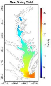
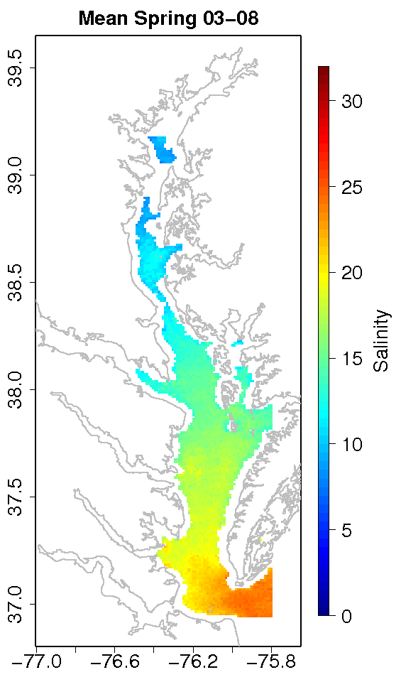
Spring Salinity Climatology for the Chesapeake

Salinity doesn’t vary that much in the open ocean, but it has a wide range in the coastal ocean. The coast is where fresh water from rivers and salt water in the ocean mix. Measurements of salinity along the coast help us understand the complex mixing between fresh and salty water and how this affects the local biology, physics, and chemistry of the seawater. However, the scope of our measurements is very small. Salinity data is collected by instruments on ships, moorings, and more recently underwater vehicles such as gliders. While these measurements are trusted to be very accurate, their spatial and temporal resolution leaves much to be desired when compared to say daily sea surface temperature estimated from a satellite in space.

So, why can’t we just measure salinity from a satellite?Well, it’s not as simple, but it is possible. NASA’s Aquarius mission http://aquarius.nasa.gov/ which was launched this past August is taking advantage of a set of three advanced radiometers that are sensitive to salinity (1.413 GHz; L-band) and a scatterometer that corrects for the ocean’s surface roughness. With this they plan on measuring global salinity with a relative accuracy of 0.2 psu and a resolution of 150 km. This will provide a tremendous amount of insight on global ocean circulation, the water cycle, and climate change. This is great new for understanding global salinity changes. What about coastal salinity? What if I wanted to know the salinity in the Chesapeake Bay? That’s much smaller than 150 km.

That’s where my project comes in. It involves NASA’s MODIS-Aqua satellite (conveniently already in orbit: http://modis.gsfc.nasa.gov/), ocean color, and a basic understanding of the hydrography of the coastal Mid-Atlantic Ocean. Here’s how it works: we already know a few things about the color of the ocean, that is, the sunlight reflecting back from the ocean measured by the MODIS-Aqua satellite. We know enough that we can estimate the concentration of the photosynthetic pigment chlorophyll-a. So not only can we see temperature from space, but we can estimate chlorophyll-a concentrations too! Anyway, there are other things in the water that absorb light besides phytoplankton and alter the colors we measure from a satellite.

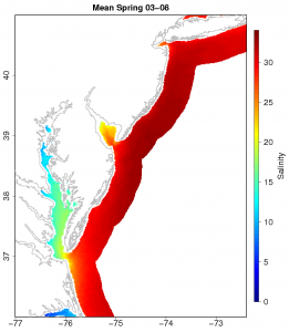
Spring Salinity Climatology for the Mid-Atlantic

We group these other things into a category called colored dissolved organic material or CDOM. CDOM is non-living detritus in the water that either washes off from land or is generated biologically. It absorbs light in the ultraviolet and blue wavelengths, so it’s detectable from satellites. In coastal areas especially, its main source of production is runoff from land. So, CDOM originates from land and we can see a signal of it from satellites that measure color. What’s that have to do with salinity?

You may have already guessed it, but water from land is fresh. So, water in the coastal ocean that is high in CDOM should be fresher than surrounding low CDOM water. Now we have a basic understanding of the hydrography of the coastal Mid-Atlantic Ocean, how it relates to ocean color, and why we need the MODIS-Aqua satellite to measure it. So, I compiled a lot of salinity data from ships (over 2 million data points) in the Mid-Atlantic coastal region (Chesapeake, Delaware, and Hudson estuaries) and matched it with satellite data from the MODIS-Aqua satellite in space and time. Now I have a dataset that contains ocean color and salinity. Using a non-linear fitting technique, I produced an algorithm that can predict what the salinity of the water should be given a certain spectral reflectance. I made a few of these algorithms in the Mid-Atlantic, one specifically for the Chesapeake Bay. It has an error of ±1.72 psu and a resolution of 1 km. This isn’t too bad considering the range in salinity in the Chesapeake is from 0-35 psu, but of course there’s always room for improvement. Even so, this is an important first step for coastal remote sensing of salinity. An algorithm like this can be used to estimate salinity data on the same time and space scale as sea surface temperature. That’s pretty useful. The folks over at the NOAA coastwatch east coast node thought so too. They took my model for the Chesapeake Bay and are now producing experimental near-real time salinity images for the area. The images can be found here: http://coastwatch.chesapeakebay.noaa.gov/cb_salinity.html. They will test the algorithm to see if it is something they want to use

Climatologies of salinity for all of my models can be downloaded here: http://modata.ceoe.udel.edu/dev/egeiger/salinity_climatologies/.

I view this project as an overall support of the NASA Aquarius mission by providing high resolution coastal salinity estimates that are rooted in in situ observations. I hope this information proves to be useful for coastal ocean modeling and understanding the complex process that effect the important resource that is our coasts.

Penguins, AUV’s, Satellites: together at last

January 21, 2011 / dw / 1 Comment

Adélie Penguin Rookery on Humble Island

Satellite tagged Adelie Penguin

Penguin swimming tracks near Palmer Station

Ballasting the Glider (Blue Hen)

Is it possible to follow penguins from space to understand where and how they are feeding in Antarctica? Absolutely!..but not without an excellent team from University of Delaware, Rutgers University, Polar Oceans Research Group, and Cal Poly San Luis Obispo. The sequence starts with the “Birders”. The “Birders” are from Polar Ocean Research and they have been studying penguins in the West Antarctic Peninsula for years. The “Birders”, headed by Bill and Donna Fraser, head out to local rookeries to identify good penguins to tag with satellite transmitters. Finding the right breeding pair is key. The pair should have two chicks with both parents still around. Some chicks only have one parent, probably because one parent was killed by a Leopard Seal. We want to choose one of the parents, because we are pretty certain they will return to their chicks to feed them. This also helps in recovering the transmitter. If the bird does not return, the transmitter comes off during their natural annual molt cycle. Once a penguin is selected, it is gently fitted with a satellite transmitter. Special waterproof tape is used to connect the transmitter to the thick feathers on the back of the penguin. The penguins are remarkably calm during the process. Once the tag is attached, the penguin is released back to its nest. The next part of the sequence is for the birds. The penguins head out to feed on krill and small fish in the area. Their tags relay their position information to ARGOS satellites and we get nightly updates. The Birders pass on their data to me nightly, and I filter and map the penguin tracks. I put them into Google Earth, so we can see where the penguins have been feeding. Then, through the magic of mathematics, we turn their tracks into predicted penguin densities. Based on these densities, we plan our AUV missions to intersect with the feeding penguins (Slocum Electric Gliders and REMUS AUV’s). The first priority is to make sure the AUV’s are ballasted correctly. This means that they need to be trimmed with weights just right so they travel correctly under the water. We use small balances and scales to get the weight of the vehicle just right, then put them into ballasting tanks to make sure we did it correctly. The vehicles should hold steady just under the surface of the water.

Getting ready for the launch of the "Blue Hen" (M. Oliver and K. Coleman)

Once we have a planned mission, we head out in small zodiacs from the station to a pre-determined point. For the Gliders, we call mission control at Rutgers University (Dave, Chip, John) and let them know a glider will be in the water shortly. Once it is in, control of the glider is accomplished via satellite telephone directly to the glider. The glider calls in and reports data and position to mission control. We can see the data coming in live over the web, and in Google Earth as we navigate the vehicle to where the penguins are feeding. The gliders move by changing their ballast, which allows them to glide up and down in the water while their wings give them forward momentum. They “fly” about 0.5mph for weeks at a time!

Mark Moline with REMUS's

In contrast to the Gliders, the REMUS vehicles are very fast and are designed for shorter, 1 day missions. Daily missions are planned around the penguin foraging locations. The Cal Poly Group (Mark Moline and Ian Robbins) have been launching 2 Remus Vehicles per day to map areas the gliders can’t get too. Like the gliders, these vehicles call back via iridium to let us know how they are doing in their mission.

MODIS Chlorophyll, Penguins, and Gliders

Glider Dances around Adélie Penguin Tracks in a sea of chlorophyll

Finally, we are getting satellite support from my lab at U.D. Erick, Megan and Danielle have been processing temperature and chlorophyll maps in near-real time to support our sampling efforts, as well as AUV operations up and down the West Antarctic Peninsula. Just today, we saw that the penguins in Avian Island (south by a few hundred miles) have been keying off of a chlorophyll front. RU05 was deployed by the L. M. Gould and will be recovered soon. All in all, it is a pretty awesome mission to track these penguins from space and AUV’s. We will see how the season develops!

Note: I will be uploading photos and videos to the ORB Lab Facebook page throughout my stay in Antarctica. Be sure to check there for my latest updates.

Penguins from Space

December 14, 2010 / dw / Comments Off

The West Antarctic Peninsula (WAP) is one of the most rapidly warming regions on Earth, with a 6°C temperature rise since 1950. Glaciers are retreating and the duration and extent of sea ice has significantly decreased. Many species rely on the sea ice as a resting platform, breeding ground, protective barrier or have life histories linked to sea ice thaw and melt cycles. With the declines in sea ice, many species are having a difficult time surviving and adapting to the new warming conditions.

The food web along the WAP is short and allows energy to be transferred efficiently. Phytoplankton (tiny plants that capture energy from the sun) are ingested by zooplankton (such as krill) which are in turn eaten by penguins, seals and whales. Due to the rapid nature of the warming around Palmer Station and the short food chain, it is an ideal location to study the effects of the acute changes in a warming environment.

Palmer Station, Antarctica

In particular, Adélie penguins are experiencing significant population declines near Palmer Station, Antarctica. On Anvers Island, populations have decreased by 70%. Declines in sea ice have also led to declines in the preferred food of Adélies. Silverfish have nearly disappeared and krill have decreased by 80%. Currently, Adélies are having a difficult time finding a satisfying meal. In turn, many species are migrating southward to look for new places to live and better food resources. On the other hand, ice-avoiding species (Gentoo and Chinstrap penguins) have been able to move south into the Adélies home range.

Adélies are a prime vertebrate species to study in relation to a changing environment. Tagging Adélies in summer breeding colonies with satellite-linked transmitters, allow foraging locations to be monitored. Their foraging tracks can be compared to satellite derived oceanic properties such as sea surface temperature, chlorophyll, sea-ice, and wind. Since conditions have changed so quickly over the last few decades, the recent development of satellites can easily detect these changes. The UD-134 Slocum Glider (underwater robot) will be deployed in January 2011 and 2012, to do additional surveys near breeding hotspots. This will allow us to combine satellite data with high resolution in-situ glider data to predict how ideal foraging locations for Adélies may change as warming continues. This will also test the satellites ability to accurately describe ecological changes that are occurring along the WAP.

Adélie Penguin

The Palmer Long Term Ecological Research Program (PAL LTER) began in 1990, and investigates aspects of this polar environment while maintaining historical records for marine species. Historical satellite data and species records will be useful in predicting phytoplankton, krill and penguin abundances and distributions. Models will be used to predict future foraging locations of Adélies in PAL LTER region of the WAP. It is important to study this region because changes are happening faster than predicted and these changes can lead to dramatic effects in our lifetimes.

Polar Orbiting Satellite Receiving Station

October 13, 2010 / dw / Comments Off

The video above is a quick screencast NASA JPL’s Eyes on the Earth application, which shows the tracks of various satellites orbiting the globe. It’s a really cool application that gives a top-notch overview of some of the satellites currently in orbit and their trajectories around the Earth. Take some time and poke around, you’ll be glad you did.

The reason I included it is that I promised to cover the polar orbiting satellite receiving station in a previous blog post about the new Satellite Receiving Station in Delaware. In the previous post I discussed the geostationary satellite receiving station. In this post, I hope to shed some light on the polar orbiting receiving setup.

What’s Inside the Radome

The equipment for the polar orbiting satellite receiving station is a bit more involved than the pretty much non-moving geostationary setup. As the name implies, the polar orbiting satellites do just that, they orbit the Earth north and south, going from pole to pole. Their path is relatively simple, they just go around the earth in circles, but as they’re doing so, the Earth is rotating beneath them. The satellites point their cameras towards the earth and essentially capture a swath of data during each rotation. Since the Earth is rotating beneath them, the swath appears as a diagonal path if you look at the overlay.

In order to capture data from a moving target, the dish has to be able to rotate and move in three axis in order to follow the satellite of interest. In order to protect the receiving equipment from the weather, it is typically installed in a circular fiberglass enclosure called a “radome”. To keep the design relatively simple, there is only one mounting configuration and radome setup created, and that’s designed to mount onboard a ship. It is then relatively simple to attach a mounting bracket to the top of a building and bolt the radome assemgly to it.

The video at the top of the page shows that there are several satellites in orbit, so the Terascan software has to pull down satellite ephemeral data from Celestrak each day, take into account the location of the tracking station, and generate a calculated schedule of which satellites will be visible to the satellite dish throughout the day. As there may be more than one satellite in view during any given time period, the satellite operator assigns a priority weighting to each satellite. The Terascan software then uses that weighting to decide which satellite it will aim the dish at and start capturing data.

Receiving Station Workstations

Inside the building is a rack of computers and receivers whose purpose in life is to control the dish on the roof of the building and to receive and process the data it relays down from the satellite. The receiving station at UD has both X and L-Band receivers which receive the data stream and pass it to a SeaSpace Satellite Acquisition Processor. The processor then sends the data packets to a Rapid Modis Processing System (RaMPS) which combines the granularized HDF data files from the satellites into a TeraScan Data File (TDF) file. Once in this format, various programs and algorithms can be run against the TDF file and channels of interest can be combined using NASA/NOAA and other user supplied algorithms to create the output product of interest. As the files can get rather large and there can be several of them coming in throughout the day, they are then moved over to a Networked Attached Storage (NAS) server and stored until they are needed.

Satellites Licensed

The UD receiving station is licensed and configured to receive data from the following satellites:

Aqua
Terra
NOAA 15
NOAA 17
NOAA 18
NOAA 19
MetOp-A (Europe)
FY-1D (China)

Hopefully this sheds a little more light on the polar orbiting receiving station and its capabilities. Let me know if there are any additions or corrections to the information I’ve posted.

New Polar and Geosynchronous Satellite Receivers for Delaware

September 26, 2010 / dw / Comments Off

A few weeks ago they fired up a new satellite receiving station from SeaSpace at the University of Delaware’s main campus in Newark, DE. Two receivers were brought online, one for L-Band reception from Geosynchronous Satellites and one for X/L-band reception from Polar Orbiting Satellites. Both receiving systems have dishes that are mounted on the roof of Willard Hall as it presented the least obstructed view of the sky. The adds additional capability to an east coast satellite operations contingent which includes:

University of Maine
City College of New York
Rutgers University
University of Delaware
University of South Florida
Louisiana State University
Purdue University

For this blog posting, I’ll only cover the geosynchronous satellite capabilities. In a future posting I’ll cover the polar orbiting hardware and its capabilities.

Geosynchronous Satellite

The beauty of geosynchronous satellites is the simplicity with which they can be tracked. Rather than flitting all about and requiring fancy calculations and equipment to track them, you merely point the dish to a point in the sky where the satellite remains fixed relative to the motion of the earth and pretty much lock the receiving dish down. Since the satellite is moving with a trajectory and speed that matches the rotation of the earth, the satellite is said to be “geo-stationary”.

The dish used to receive the signals from the geosynchronous satellites is therefore simple in its design. It is mounted with only one axis of movement, meaning it can only be adjusted along an arc of the sky either to the east or to the west. There is a motor and lead screw mounted on the back that will either push the dish one way, or pull the dish the other in order to position it for the best signal strength. The current intent of the UD dish seems to be dedicated to constantly receiving real-time data from the GOES-EAST satellite (also known as “GOES-13”). GOES East outputs full disk imagery of the the earth from a longitude of 75 degrees west, which gives a good view of pretty much all of North and South America and a good chunk of the Pacific and Atlantic Ocean.

GOES stands for “Geostationary Operational Environmental Satellite” and it is operated by NOAA’s NESDIS or “National Environmental Satellite, Data, and Information Service” primarily to support meteorological operations and research, which includes weather forecasting and storm tracking. The dish is oriented in such a way that it could also be programmed to point to GOES-WEST (aka GOES-11) for a satellite view of the Pacific Ocean (centered around 135 degrees west longitude) as well if the need arises.

GOES Sensors

One thing to bear in mind is that GOES-13 hasn’t always been “GOES East” – it took over for GOES-12 in April 2010, with GOES-12 moving to 60 degrees West to replace GOES-10 (decommissioned) for coverage of South America. I note this so that you don’t assume that the sensors (and/or their calibration factors) for a particular GOES station are always the same.

Imager

The current GOES-East has optical imagers with 6 channels with resolutions of 1.1km for the visible channel (one); and 4km and 8km resolutions for the near infrared, water vapor and thermal infrared channels (two through six). The imager is basically a rotating mirror and lens configuration that scans the earth from north to south, line by line to receive reflected visible light, water vapor as well as infrared radiation channels. Each line scanned is digitized and transmitted back towards the earth with measurement units of percent albedo for visible light and temperature for the water vapor and infrared information. Spectral response functions can now also be downloaded online from the NOAA Office of Satellite Operations as well as other GOES calibration information.

Sounder

GOES satellites are also equipped with a sounder with 8km resolution. The sounder scans the atmosphere over the land and ocean and provides vertical profiles which include the temperature of the surface and cloud tops as well as derived wind velocities from these measurements.

Real-time Access to Data

The key feature to having a satellite receiving station on-site is the access to the raw, real-time satellite data. Sure, you can get pull some images down from the NOAA Geostationary Satellite Server, but they would be just derived images. Scientists here at UD and elsewhere are interested in getting the latest raw data feeds from the satellites so that they can research and develop algorithms that process the raw channel data into other products in support of their research projects.

Next on my agenda is to try to give some insight into the polar orbiting satellite tracking station and the fancy gear that sits inside the radome enclosure. Cheers!

Turning Satellite Data into Google Earth Maps: It’s Easy!

August 21, 2010 / dw / 3 Comments

As a new grad student in the ORB (Ocean exploration, Remote Sensing, and Biogeography) lab at the University of Delaware under Dr. Matthew Oliver, I (along with my cohort Danielle Haulsee) were tasked with learning to write code in R. R is a language that enables statistical computing and making graphical displays. To some of you this may sound basic, but having no prior programming experience it was a little overwhelming at times. After getting the basics down, we then started pulling sea surface temperature and chlorophyll data from NASA’s Goddard Space Flight Center (GSFC) MODIS Aqua satellite. This isn’t just any temperature and chlorophyll data either, it’s real-time and updated everyday! From this we were able to create maps on Google Earth, which is a great platform for viewing and interacting with multiple data layers on a global scale. This allows us to easily distribute NASA’s data for ocean planning. These overlays along with others were also able to assist in planning Slocum Glider missions in areas surrounding the Gulf oil spill.

In our Google Earth maps, we created 1, 3, and 8 day averages that reflect the current conditions in the ocean. Each day our code downloads the lastest satellite data that has been updated on NASA’s website and then it is averaged along with the previous days to create an average. The 1 day average maps are patchy due to the fact that the satellites can not see through the clouds. Therefore, the 8 day averages make for a more complete and accurate picture. For higher resolution images, we created smaller maps of just California, the East Coast and even Antarctica! These locations correspond to areas that we conduct further research in. Google Earth was interested in our overlays so check out the Google Earth Gallery for sea surface temperature and chlorophyll concentrations near you!